

About
Agent Boutique AI’s client work spans the media domain. Speech models show up often enough that “we’ll figure it out later” stops working as a strategy. So we run Wise Wednesdays, a standing internal series for closing gaps like that. The rule is simple: pick a topic, and spend as long as it takes to actually understand it. No skimming a blog post and moving on.
Speech recognition is the most recent run of that series. It’s the one worth writing up.
It took six sessions, longer than most. One question kept coming back: why does a live transcript feel like it’s thinking harder the longer someone talks?
Chasing that question took us from the physics of sound all the way to a 2026 streaming-ASR paper. That’s the arc this post follows. Want the original slides? Download the presentation (PDF).
The demo that kicked it off
It started as a demo, not a lecture. One of our engineers walked us through Little Voices, with the tagline: “Made with Love for Kids (Human Taste + AI Execution).” It was built using AI tooling, guided by completely human taste.
It’s a local-only journaling tool, built for his kids. The younger one had started keeping a diary at school. He knew the words he wanted to write, but not how to spell them. “Vent” for “went” was the example that came up. He didn’t want to ask an adult every time.
So the tool listens. It transcribes what a child says, locally, so nothing leaves the device. And it highlights each word as it’s spoken, so the child can check the spelling themselves.
The interesting engineering choice was already there in that first demo. The app runs two different model sizes for two different jobs.
A small, fast Whisper model transcribes live, word by word, keeping up with speech as it happens. Once the recording stops, a larger, slower model re-transcribes the whole clip for the version that gets saved.
Speed where the user is watching. Accuracy where it counts.
That split also surfaced the first real bug: hallucination on silence.
Whisper was trained on hundreds of thousands of hours of scraped audio, much of it from YouTube. Feed it dead air, or a fan hum, and it doesn’t stay quiet. It says things like “Thank you for watching” or “Don’t forget to subscribe.” Why? Because that’s what usually follows a silent pause in its training data.
For an app transcribing a seven-year-old’s diary, that’s not a quirk. It’s a correctness bug.
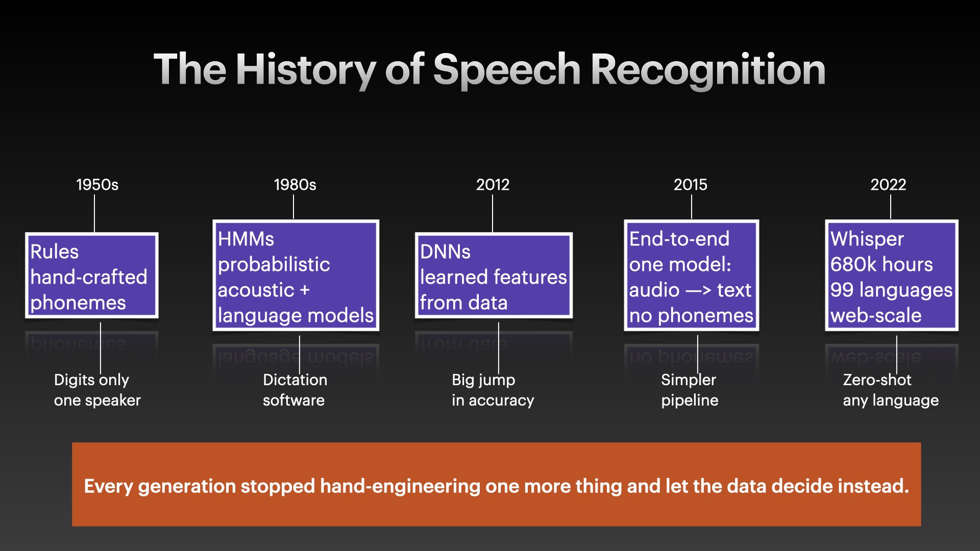
And it’s the thread that pulled us into everything that came next. You can’t reason about a model’s failures until you understand what it was trained on, and how it turns sound into text in the first place.
Sound is just numbers, and the numbers you pick matter
The next session started from first principles. It’s worth spelling these out plainly, because they quietly control everything downstream.
A microphone turns air pressure into voltage. An analog-to-digital converter samples that voltage thousands of times a second, turning it into a list of integers. Three parameters define the result:
| Parameter | Controls | Little Voices’ choice | Why |
|---|---|---|---|
| Sample rate | How often you measure | 16,000 Hz | Human speech tops out around 8 kHz. Nyquist’s rule says you need double that to reconstruct it losslessly, so 16 kHz. Whisper was trained on 16 kHz audio too, so there’s no benefit going higher. |
| Bit depth | How precisely you measure | 16-bit | That’s 65,536 discrete levels of precision. Plenty for clean voice. Going higher is overkill for speech. |
| Channels | How many microphones | Mono | ASR models throw away spatial information anyway. Stereo would double the data for no benefit. |
Those three numbers set the data rate. One minute of audio comes out to about 1.9 MB. That’s small, but it adds up fast over a WebSocket connection streaming continuously. So the format matters too.
Live audio moves as raw PCM bytes, just a flat list of integers, with zero overhead. When it’s saved, a 44-byte WAV header gets added on top, so any player can read it. For long-term storage, or emailing a recording to a parent, it gets re-encoded as FLAC. FLAC losslessly compresses the stream to roughly half the size, by storing the differences between adjacent samples instead of the raw values.
The hallucination problem from the first session has a fix that lives right here: Voice Activity Detection.
We run a VAD pass (the Silero model, via faster-whisper) before transcription. Silence, fan noise, and breathing never reach the decoder at all. If there’s no speech, there’s nothing for the model to hallucinate a caption for.
The trade-off is latency versus completeness. VAD is on for the final, accuracy-focused pass. It’s off during live transcription, where the priority is showing something on screen right away, and correcting it later.
Silence detection is a filter you can only afford to skip if you’re not the one who has to decide what’s true.
flowchart LR
    A[Microphone] -->|Pressure wave| B[Raw PCM<br/>16kHz / 16-bit / mono]
    B -->|Live, ~100ms chunks| C[Small model<br/>beam=1, temp=0, VAD off]
    B -->|On save| D[Large model<br/>beam=5, VAD on]
    C --> E[Live word highlighting]
    D --> F[Final saved transcript]
What Whisper actually does with those samples
Whisper doesn’t see waveforms. It sees pictures.
Raw PCM, 16,000 numbers a second, is hard to learn from. Too dense. No structure a convolution can grab onto. So the pipeline turns it into an image instead:
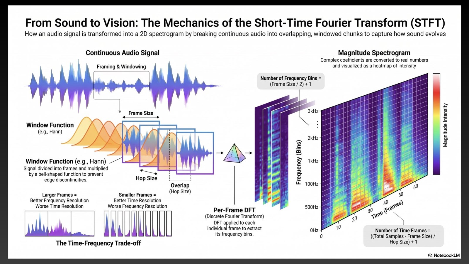
- Short-Time Fourier Transform (STFT). The signal gets sliced into overlapping 25ms windows (400 samples at 16 kHz), with a 10ms hop between them. Each window is shaped by a Hann function, which avoids the noise a hard rectangular cut would introduce. Then each window gets its own frequency breakdown, via a per-frame DFT. Why 25ms? It’s a deliberate trade-off, not a default. Shorter windows lose some frequency resolution, but sharpen timing. And timing is what you need to tell a “t” from a “d”: consonants that differ only in the first few milliseconds of sound. Longer windows do the opposite.
- Mel filterbank + log scale. The raw STFT output has thousands of frequency bins, and most go to waste. Human hearing resolves low frequencies far more precisely than high ones, so the Mel scale compresses accordingly. Then there’s volume. The energy difference between a whisper and a shout is roughly a million to one. A log transform squashes that whole range down to something like 0–6. That way quiet and loud speech become equally learnable, instead of one drowning out the other.
The result, for 30 seconds of audio, is an 80-bin by 3,000-frame image: the log-Mel spectrogram. This is genuinely what Whisper “sees.” Not the sound. A picture of the sound.
From there, it’s a standard encoder-decoder Transformer. The encoder reads the spectrogram. The decoder generates text tokens one at a time. Cross-attention links the two together.
Two design choices here are worth calling out, because they explain a lot of what happens downstream:
- Multitask via special tokens, not separate models. One Whisper checkpoint handles transcription, translation, and language ID. The task is just another token in the input sequence.
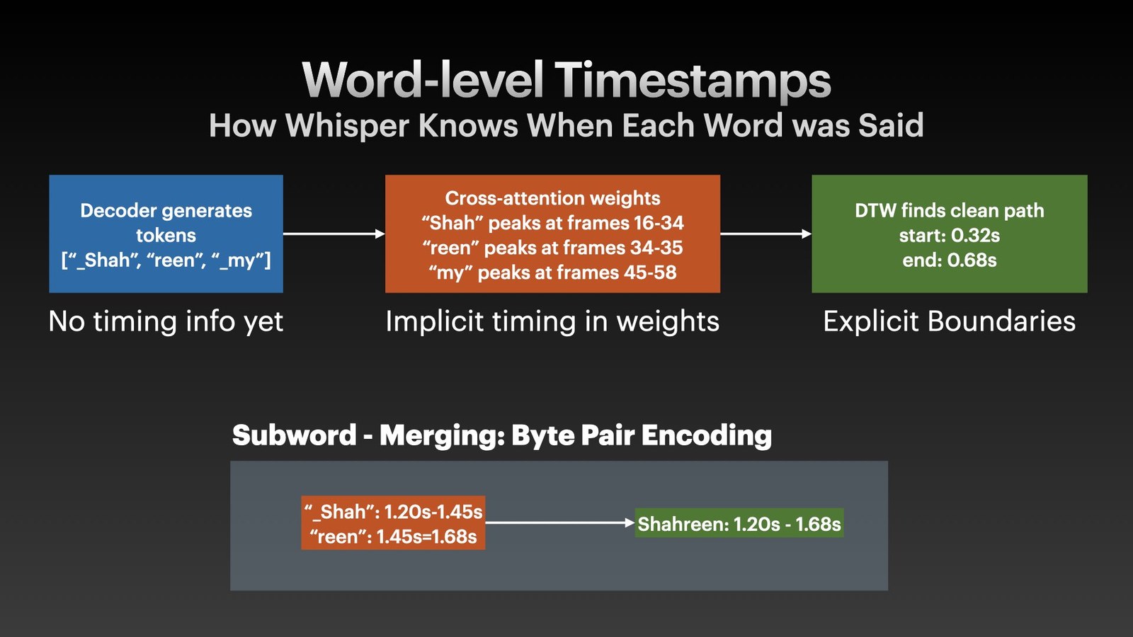
<|te|><|transcribe|>and<|te|><|translate|>steer the exact same weights toward different outputs. That’s a simpler pipeline than the old era of separate acoustic, language, and translation models. The cost: the model only knows what task it’s doing because you told it, explicitly, up front. - Word timestamps are recovered, not predicted directly. As the decoder emits sub-word tokens, its cross-attention weights spike over specific spectrogram frames. Attention naturally lines up with where in the audio a token “came from.” Running dynamic time warping over those attention weights turns that loose alignment into hard start and end boundaries, per token. Byte-pair merging then stitches sub-word pieces ("_Shah" plus “reen”) back into whole words, with a combined time range. It’s a clever reuse of a mechanism built for something else entirely, and it’s the reason Little Voices can highlight the exact word a child is listening back to.
Speed versus accuracy shows up again at decode time. It’s the same dial the app already uses elsewhere.
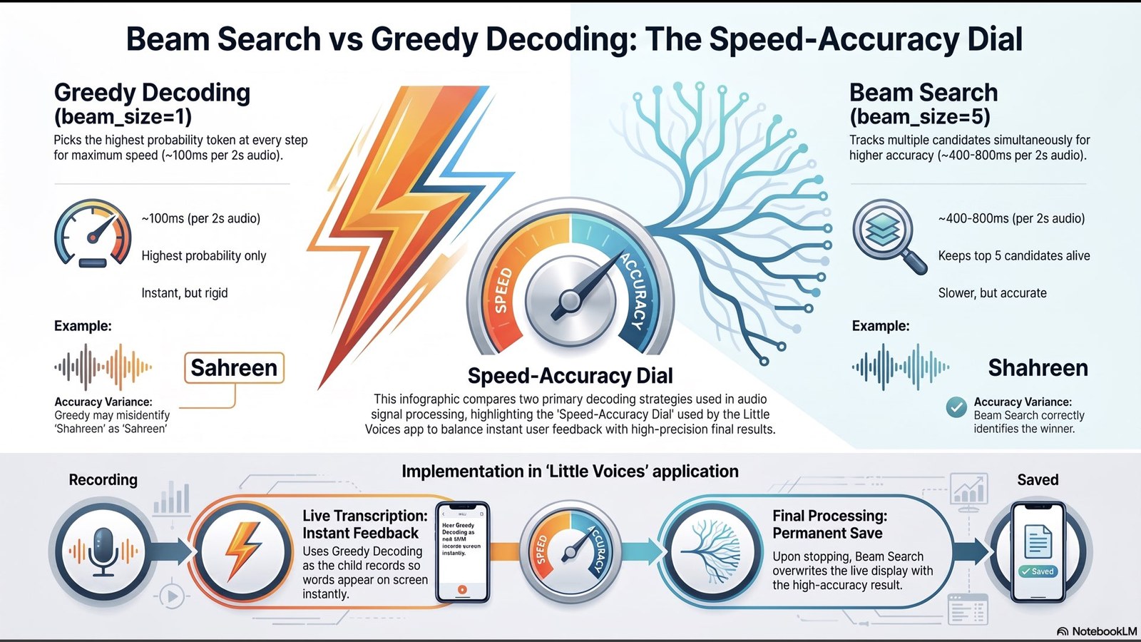
Greedy decoding (beam_size=1) picks the single highest-probability token at every step. It’s fast, about 100ms for 2 seconds of audio, but rigid enough to occasionally lock in “Sahreen” when the correct word was “Shahreen.”
Beam search (beam_size=5) tracks five candidate sequences at once, and picks the best one at the end. That takes longer, 400 to 800ms for the same clip, but it catches the correction greedy decoding commits to too early.
Live transcription uses greedy, for instant feedback. The final save re-runs everything with beam search.
Temperature is pinned to 0.0 for live transcription too. That stops the model from amplifying uncertainty into random text: a second defense against hallucination, alongside VAD.
The wall: why “wait for the whole clip” doesn’t scale to streaming
Everything so far explains Whisper well. It also explains why Whisper is an awkward fit for anything that has to respond while someone is still talking.
Two structural facts collide here.
Whisper’s encoder uses global full attention. Every frame of the spectrogram attends to every other frame. That’s exactly what gives it strong contextual accuracy: distant context helps resolve locally ambiguous sounds.
But self-attention cost scales as O(N²) with sequence length. Worse, the encoder can’t hand off a single token until it’s processed the entire input. Whisper’s answer is to just fix the length: audio gets chunked into rigid 30-second windows, padded if it’s shorter.
That’s a fine trade for offline, batch transcription. It’s a bad one for streaming. Time-to-first-token is tied to how much audio you’ve already collected. The longer the buffered clip, the longer the wait before the first word appears, growing without bound as more audio piles up.
Humans don’t grant much patience for that wait. There’s a well-known threshold, around 250ms, past which a response stops feeling instant and starts feeling laggy. Press a button. If the UI reacts within 250ms, you don’t notice. Past it, you do.
It’s the same wall Spotify famously ran into, a story retold in Netflix’s The Playlist. They wanted a song to start playing the instant you hit play. But a TCP connection’s handshake and acknowledgment, the round trip alone, eats up around 250ms before the first packet of audio even arrives. That’s physics, not a bug. It’s part of why they moved to UDP, trading delivery guarantees for the ability to just start playing.
Speech itself is forgiving in a way full-attention models don’t take advantage of. A syllable spans roughly 150 to 350ms of sound, and a human listener doesn’t need to hear the end of a sentence to start parsing its beginning.
Full-attention ASR does the opposite. It insists on seeing the entire utterance before it commits to a first token. That’s a mismatch between how the model reasons and how speech, and listening, actually unfold in time.
We modeled what that mismatch costs. On a representative edge-class device (about 0.5 TOPS), a full-attention encoder’s time-to-first-token breaches the 250ms threshold once the buffered clip hits roughly four seconds. That’s well within a single sentence.
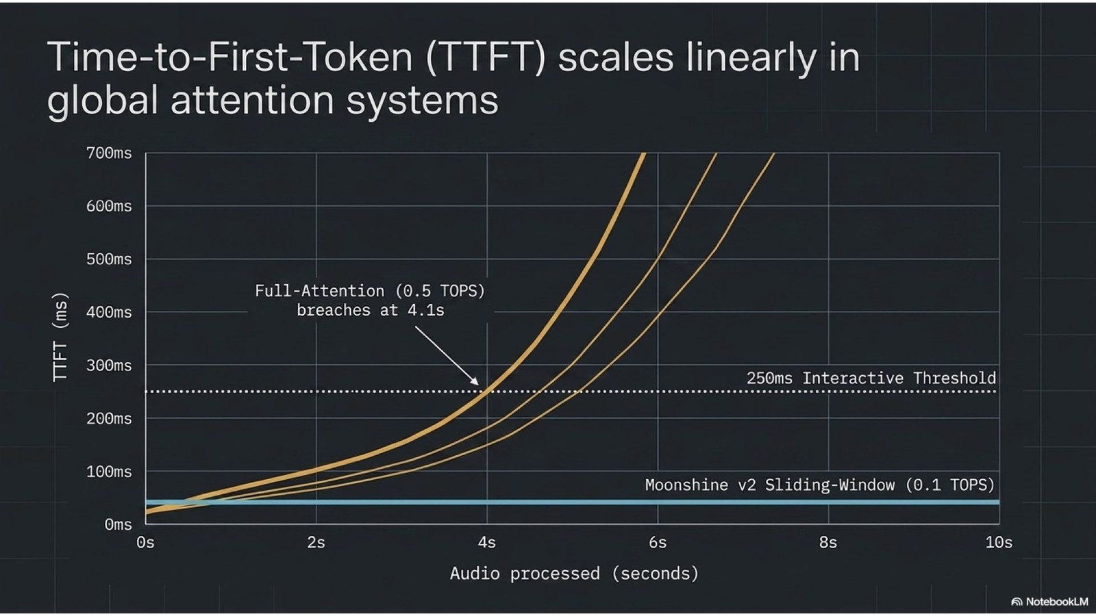
Past that point, every extra second of audio makes the wait longer, not shorter. That’s the exact opposite of what live captioning or a voice assistant needs.
Moonshine v2: bound the window instead of widening it
The fix comes from the Moonshine v2 paper, “Ergodic Streaming Encoder ASR for Latency-Critical Speech Applications.” It doesn’t try to make full attention faster. It removes the reason full attention was slow in the first place.
Instead of every frame attending to every other frame in the whole clip, the encoder uses sliding-window self-attention. Each frame attends only to a fixed local window: 16 frames of left (past) context, and up to 4 frames of right (near-future) context.
That window size isn’t arbitrary. At the model’s 50 Hz frame rate, 16 frames works out to 320ms, and 4 frames to 80ms. That’s chosen on purpose: it comfortably covers a full syllable (150 to 350ms), with a little slack left over to resolve a word that was still incomplete when the window closed.
There’s a nice symmetry here. He’d already been teaching his kids to sound out spellings by clapping out syllables. “Today” becomes two claps: “to” and “day,” each decoded separately. That’s an intuitive, human-scale way of chunking speech into pieces small enough to reason about one at a time.
Moonshine v2 encodes almost the identical idea into its architecture. Don’t try to reason about the whole utterance at once. Reason about one syllable-sized window at a time.
The result is a real complexity change, not just a constant-factor speedup. Cost drops from O(N²) to O(N·w), where w is the fixed window size. That’s linear in audio length.
More important for streaming: the encoder is ergodic. It carries no positional embeddings, and it does the exact same computation no matter where in the stream a window sits. It genuinely cannot tell the difference between the start of a recording and its ten-thousandth second. Memory usage and per-window latency stay flat, no matter how long the stream runs.
The decoder still needs positional information to produce coherent sentences, though. So an adapter reintroduces it downstream: it stamps rotary positional embeddings onto the encoder’s position-free output, before handing off to a standard causal, autoregressive decoder.
Worth being honest about that decoder: it’s still the bottleneck the encoder redesign never touched. Sequential, autoregressive generation doesn’t parallelize the way the new encoder does. We flagged this as the next thing worth investigating: whether faster decoding strategies from other model families (Parakeet’s transducer-style decoding came up) could be adapted here too.
flowchart TD
    subgraph Whisper["Whisper: full attention"]
        direction LR
        A1[Frame 1] <--> A2[Frame 2] <--> A3[...] <--> A4[Frame N]
        note1["Every frame attends to every frame.<br/>O(N²). Must see the whole 30s clip<br/>before the first token."]
    end
    subgraph Moonshine["Moonshine v2: sliding window"]
        direction LR
        B1[16 frames<br/>past] --> B2[current<br/>frame]
        B3[4 frames<br/>future] --> B2
        note2["Fixed window per frame.<br/>O(N·w). Constant lookahead,<br/>constant memory, any stream length."]
    end
We ran our own local comparison too, testing Whisper large-v3, Moonshine, Parakeet-TDT, and Canary-Qwen side by side on the same clip. Even before the formal numbers came in, the direction was clear: Moonshine’s real-time factor came in at roughly a quarter of Whisper’s, with Parakeet’s transducer decoder faster still.
The paper puts a firmer number on it. On identical hardware, an Apple M3, Moonshine v2 Medium responds in 258ms. Whisper Large v3 takes 11,286ms. That’s a 43.7x difference, using well under a tenth of the compute.
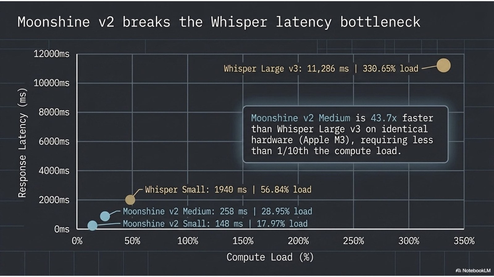
It gets there at 245M parameters, against Whisper Large’s 1.5B, roughly a sixth the size. And the paper reports accuracy competitive with models many times larger. Not a free lunch, though: real-time speed here does cost some accuracy against the largest Whisper checkpoint. Just not much.
Why the trade makes sense for some things and not others
None of this makes Moonshine strictly “better” than Whisper. It optimizes for a different point on the same curve.
Full attention’s contextual accuracy is a real advantage when nothing is waiting on the first token: podcast transcripts, meeting recordings, archival captioning. A bounded, position-free encoder earns its keep when something is waiting while the person is still talking: a live caption, a local voice assistant, an on-device tool for a child’s diary that has to feel responsive to be usable at all.
That profile also happens to match what privacy-sensitive, on-device applications need: small enough, and light enough on compute, to run entirely on the hardware in front of you, with no round trip to a server. That’s a second reason it fits the constraints Little Voices was built under, on top of the raw speed win.
What the series was actually for
Six sessions to get from “why does my kid’s transcription app say weird things during silence” to “here’s the algorithmic reason full attention doesn’t stream well, and here’s the paper that fixes it.” That’s not a fast path.
But it’s the right amount of time, we think, before you treat any of this as settled knowledge you’d build a client-facing system on. The Wise Wednesdays format is deliberately unhurried. Read the material. Sit with it for a week. Come back with real questions. Let one topic run as many sessions as it needs, instead of compressing it into a single deck.
One habit worth stealing, if you try something similar: while you’re waiting on any long-running generation task (our example was having an agent build side-by-side prototypes of competing libraries), read the primary documentation in parallel instead of just waiting.
You get two independent passes at the same question: one from the docs, one from a working example. They tend to disagree in useful places.